gsDesignCRT example

Introduction

This article outlines the procedure for calculating the maximum and expected sample sizes and then evaluating the corresponding empirical power via simulation for a parallel group sequential CRT using the gsDesignCRT package.

Calculating maximum and expected sample sizes

Suppose we were to design a group sequential CRT with continuous outcomes and $K = 3$ interim analyses where two-sided tests for early efficacy or binding futility stopping are conducted. We want to calculate the maximum number of clusters per arm $m_{max}$ needed to detect an effect size of $0.2$ with $0.05$ Type I error and $0.9$ power assuming the variance of outcomes in both arms is $1$, the intracluster correlation coefficient (ICC) is $0.1$, and the average cluster size is $50$ participants. For calculating the expected number of participants per arm, we will assume that recruitment will be conducted with $m_{max}$ clusters enrolled at the beginning of the trial with individual participants recruited into the clusters over time.

library(gsDesignCRT)

## Specify desired population parameters and error rates
mu_vec <- c(0, 0.2) # Mean outcome for intervention arms
sd_vec <- c(1, 1) # Standard deviations for intervention arms
delta <- abs(mu_vec[2] - mu_vec[1]) # Desired effect size; must be > 0
n <- 50 # Average cluster size
rho <- 0.1 # ICC

alpha <- 0.05 # Type I error
beta <- 0.1 # Type II error (1 - power)

## Specify how interim analyses are conducted
k <- 3 # number of interim analyses
test_type <- 4 # efficacy or binding futility stopping
test_sides <- 2 # two-sided test
size_type <- 1 # calculate maximum number of clusters per arm m_max
recruit_type <- 2 # recruit individuals within clusters
timing_type <- 2 # calculate maximum sample size based on information
# increments in info_timing but calculate expected sample size based on sample
# increments in size_timing
alpha_sf <- sfLDOF # Efficacy bound spending function (O'Brien-Fleming here)
beta_sf <- sfLDOF # Futility bound spending function (O'Brien-Fleming here)

## Calculate corresponding sample size
size_calc <- gsDesignCRT(k = k,
                         outcome_type = 1, # continuous outcomes
                         test_type = test_type,
                         test_sides = test_sides,
                         size_type = size_type,
                         recruit_type = recruit_type,
                         timing_type = timing_type,
                         delta = delta,
                         sigma_vec = sd_vec,
                         rho = rho,
                         alpha = alpha,
                         beta = beta,
                         n_fix = n,
                         info_timing = 1,
                         size_timing = 1,
                         alpha_sf = alpha_sf,
                         beta_sf = beta_sf)

# Maximum number of clusters per arm
size_calc$max_m
#> [1] 64.5923

# Maximum total number of participants
size_calc$max_total
#> [1] 6459.23

# Expected total number of participants under null and alternative hypotheses
size_calc$e_total
#> [1] 2586.719 2751.012

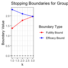
Evaluating empirical power via simulations

After calculating the maximum sample size, suppose we want to evaluate the empirical power of the corresponding trial. We assume that interim analyses are conducted with a Z-test where variance and ICC are re-estimated at each analysis, participants are recruited exactly according to how the analyses were originally scheduled, and stopping boundaries are re-computed using the observed information at each analysis.

set.seed(3)

## Specify simulation parameters
stat_type <- 2 # Z-test with re-estimated variance and ICC
balance_size <- 1 # Exact sample increments according to the scheduled analyses
precompute <- FALSE # Re-compute stopping boundaries using observed information
# at each analysis

## Conduct simulations
reject <- c()

for (i in 1:1000) {
  sim_df <- genContCRT(m = ceiling(size_calc$max_m), n = n,
                       mu_vec = mu_vec, sigma_vec = sd_vec, rho = rho)
  sim_trial <- gsSimContCRT(k, data = sim_df,
                            test_type = test_type, test_sides = test_sides,
                            recruit_type = recruit_type, stat_type = stat_type,
                            balance_size = balance_size,
                            precompute = precompute,
                            delta = delta, rho = rho,
                            alpha = alpha, beta = beta,
                            m_max = ceiling(size_calc$max_m), n_max = n,
                            alpha_sf = alpha_sf, beta_sf = beta_sf)
  reject <- c(reject, sim_trial$reject)
}

## Estimate empirical power from simulations
mean(reject)
#> [1] 0.88